Trigonometry Vocabulary
Key Terms and Definitions
- **Angle**: The space (usually measured in degrees or radians) between two intersecting lines or surfaces at or close to the point where they meet.
- **Acute Angle**: An angle that is less than \( 90^\circ \).
- **Obtuse Angle**: An angle that is greater than \( 90^\circ \) but less than \( 180^\circ \).
- **Right Angle**: An angle of exactly \( 90^\circ \).
- **Radians**: A measure of angle size, defined such that there are \( 2\pi \) radians in a complete circle.
- **Reference Angle**: The smallest angle between the terminal side of the given angle and the x-axis, always positive.
- **Sine Function \( \sin \theta \)**: In a right triangle, the ratio of the opposite side to the hypotenuse.
- **Cosine Function \( \cos \theta \)**: In a right triangle, the ratio of the adjacent side to the hypotenuse.
- **Tangent Function \( \tan \theta \)**: The ratio of the opposite side to the adjacent side in a right triangle; it is also equal to \( \frac{\sin \theta}{\cos \theta} \).
- **Secant Function \( \sec \theta \)**: The reciprocal of the cosine function, i.e., \( \sec \theta = \frac{1}{\cos \theta} \).
- **Cosecant Function \( \csc \theta \)**: The reciprocal of the sine function, i.e., \( \csc \theta = \frac{1}{\sin \theta} \).
- **Cotangent Function \( \cot \theta \)**: The reciprocal of the tangent function, i.e., \( \cot \theta = \frac{1}{\tan \theta} \).
- **Unit Circle**: A circle with radius 1, centered at the origin of a coordinate plane, used to define the trigonometric functions.
- **Quadrants**: The four regions of the coordinate plane, determined by the x-axis and y-axis.
- **Trigonometric Identity**: A true statement that involves trigonometric functions and is valid for all values of the variable (e.g., \( \sin^2 \theta + \cos^2 \theta = 1 \)).
- **Periodic Function**: A function that repeats its values in regular intervals or periods.
- **Inverse Trigonometric Functions**: Functions that give the angle corresponding to a given trigonometric ratio (e.g., \( \sin^{-1} \), \( \cos^{-1} \), \( \tan^{-1} \)).
- **Complementary Angles**: Two angles whose measures sum to \( 90^\circ \).
- **Supplementary Angles**: Two angles whose measures sum to \( 180^\circ \).
Trigonometric Ratios for Angles Between \(0^\circ\) and \(90^\circ\)
Trigonometric Ratios
For a right triangle with an angle \( \theta \), the following trigonometric ratios apply:
\[ \sin \theta = \frac{\text{opposite}}{\text{hypotenuse}} \] \[ \cos \theta = \frac{\text{adjacent}}{\text{hypotenuse}} \] \[ \tan \theta = \frac{\text{opposite}}{\text{adjacent}} \]
In terms of coordinates in a right triangle, we define:
- x: adjacent side
- y: opposite side
- r: hypotenuse
Worked Example
Hint: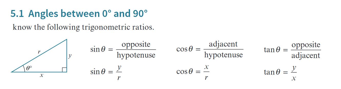
Given:
\[ \cos \theta = \frac{\sqrt{5}}{3}, \quad \text{where } 0^\circ \leq \theta < 90^\circ \]
a. Find the exact values of:
i. \( \cos^2 \theta \)
Using the definition of \( \cos \theta \):
\[ \cos^2 \theta = \left(\frac{\sqrt{5}}{3}\right)^2 = \frac{5}{9} \]
ii. \( \sin \theta \)
Using Pythagoras’ theorem in the right triangle:
\[ \text{If } r = 3, \text{ then } x = \sqrt{5}, \text{ and } y = \sqrt{r^2 - x^2} = \sqrt{3^2 - \left(\sqrt{5}\right)^2} = \sqrt{9 - 5} = \sqrt{4} = 2 \]
Thus:
\[ \sin \theta = \frac{y}{r} = \frac{2}{3} \]
iii. \( \tan \theta \)
From the triangle:
\[ \tan \theta = \frac{\text{opposite}}{\text{adjacent}} = \frac{y}{x} = \frac{2}{\sqrt{5}} \]
Additional Notes
The expression \( \cos^2 \theta \) means \( (\cos \theta)^2 \), indicating the square of the cosine of angle \( \theta \).
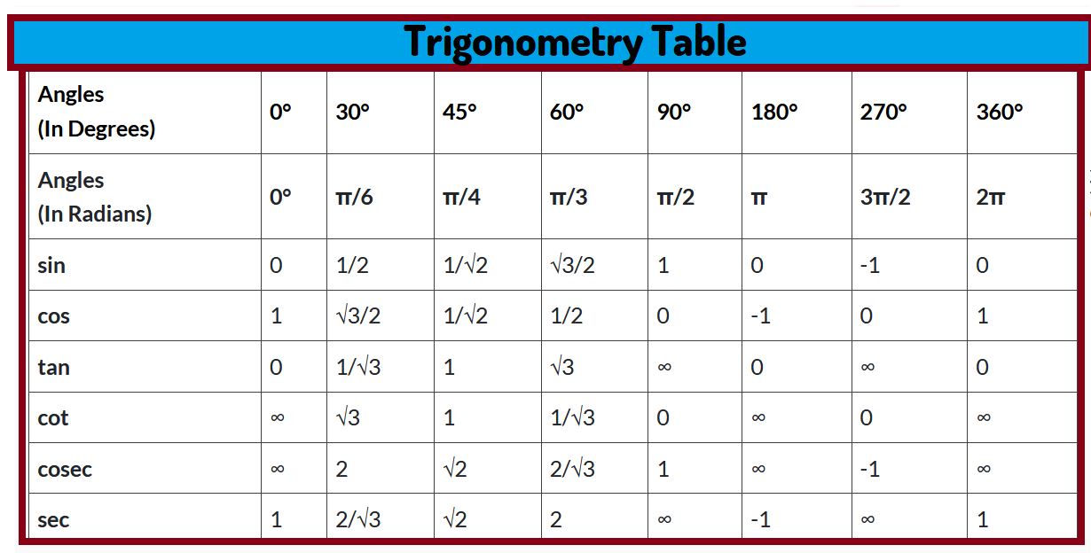
Trigonometry Table: Things to Remember
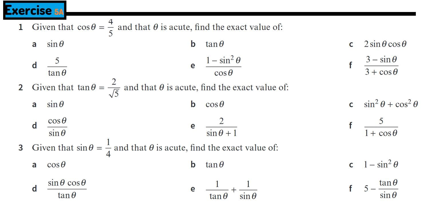
Exercise 5A Solutions
1. Given that \( \cos \theta = \frac{4}{5} \) and that \( \theta \) is acute, find the exact value of:
a. \( \sin \theta \)
Since \( \cos^2 \theta + \sin^2 \theta = 1 \), we have: \[ \sin^2 \theta = 1 - \cos^2 \theta = 1 - \left(\frac{4}{5}\right)^2 = 1 - \frac{16}{25} = \frac{9}{25} \] Therefore: \[ \sin \theta = \frac{3}{5} \]
b. \( \tan \theta \)
We know: \[ \tan \theta = \frac{\sin \theta}{\cos \theta} = \frac{\frac{3}{5}}{\frac{4}{5}} = \frac{3}{4} \]
c. \( 2 \sin \theta \cos \theta \)
Using the formula for \( \sin 2\theta \), we have: \[ 2 \sin \theta \cos \theta = 2 \times \frac{3}{5} \times \frac{4}{5} = \frac{24}{25} \]
d. \( \frac{5}{\tan \theta} \)
Since \( \tan \theta = \frac{3}{4} \), we have: \[ \frac{5}{\tan \theta} = \frac{5}{\frac{3}{4}} = \frac{5 \times 4}{3} = \frac{20}{3} \]
e. \( \frac{1 - \sin^2 \theta}{\cos \theta} \)
Since \( 1 - \sin^2 \theta = \cos^2 \theta \), we have: \[ \frac{1 - \sin^2 \theta}{\cos \theta} = \frac{\cos^2 \theta}{\cos \theta} = \cos \theta = \frac{4}{5} \]
f. \( \frac{3 - \sin \theta}{3 + \cos \theta} \)
Substituting \( \sin \theta = \frac{3}{5} \) and \( \cos \theta = \frac{4}{5} \), we get: \[ \frac{3 - \sin \theta}{3 + \cos \theta} = \frac{3 - \frac{3}{5}}{3 + \frac{4}{5}} = \frac{\frac{15}{5} - \frac{3}{5}}{\frac{15}{5} + \frac{4}{5}} = \frac{\frac{12}{5}}{\frac{19}{5}} = \frac{12}{19} \]
2. Given that \( \tan \theta = \frac{2}{\sqrt{5}} \) and that \( \theta \) is acute, find the exact value of:
a. \( \sin \theta \)
We know \( \tan \theta = \frac{\sin \theta}{\cos \theta} \), and since \( \tan \theta = \frac{2}{\sqrt{5}} \), let’s first find \( \cos \theta \) using: \[ \sin^2 \theta + \cos^2 \theta = 1 \] \[ \frac{\sin \theta}{\cos \theta} = \frac{2}{\sqrt{5}} \] Substituting this back, we get: \[ \sin^2 \theta = \frac{4}{9}, \quad \sin \theta = \frac{2}{3} \]
b. \( \cos \theta \)
Using the relationship \( \sin^2 \theta + \cos^2 \theta = 1 \), we can find: \[ \cos^2 \theta = 1 - \frac{4}{9} = \frac{5}{9}, \quad \cos \theta = \frac{\sqrt{5}}{3} \]
c. \( \sin^2 \theta + \cos^2 \theta \)
We know: \[ \sin^2 \theta + \cos^2 \theta = 1 \]
d. \( \frac{\cos \theta}{\sin \theta} \)
Using the value of \( \sin \theta \) and \( \cos \theta \), we get: \[ \frac{\cos \theta}{\sin \theta} = \frac{\frac{\sqrt{5}}{3}}{\frac{2}{3}} = \frac{\sqrt{5}}{2} \]
e. \( \frac{2}{\sin \theta + 1} \)
Substituting \( \sin \theta = \frac{2}{3} \), we get: \[ \frac{2}{\sin \theta + 1} = \frac{2}{\frac{2}{3} + 1} = \frac{2}{\frac{5}{3}} = \frac{6}{5} \]
f. \( \frac{5}{1 + \cos \theta} \)
Substituting \( \cos \theta = \frac{\sqrt{5}}{3} \), we get: \[ \frac{5}{1 + \cos \theta} = \frac{5}{1 + \frac{\sqrt{5}}{3}} = \frac{5 \times 3}{3 + \sqrt{5}} = \frac{15}{3 + \sqrt{5}} \]
3. Given that \( \sin \theta = \frac{1}{4} \) and that \( \theta \) is acute, find the exact value of:
a. \( \cos \theta \)
Using the identity \( \sin^2 \theta + \cos^2 \theta = 1 \), we can find: \[ \cos^2 \theta = 1 - \sin^2 \theta = 1 - \left( \frac{1}{4} \right)^2 = 1 - \frac{1}{16} = \frac{15}{16} \] Therefore: \[ \cos \theta = \frac{\sqrt{15}}{4} \]
b. \( \tan \theta \)
We know \( \tan \theta = \frac{\sin \theta}{\cos \theta} \), so: \[ \tan \theta = \frac{\frac{1}{4}}{\frac{\sqrt{15}}{4}} = \frac{1}{\sqrt{15}} \]
c. \( 1 - \sin^2 \theta \)
Since \( 1 - \sin^2 \theta = \cos^2 \theta \), we have: \[ 1 - \sin^2 \theta = \frac{15}{16} \]
d. \( \frac{\sin \theta \cos \theta}{\tan \theta} \)
We know: \[ \frac{\sin \theta \cos \theta}{\tan \theta} = \sin \theta \cdot \cos \theta \] Substituting \( \sin \theta = \frac{1}{4} \) and \( \cos \theta = \frac{\sqrt{15}}{4} \), we get: \[ \sin \theta \cdot \cos \theta = \frac{1}{4} \times \frac{\sqrt{15}}{4} = \frac{\sqrt{15}}{16} \]
e. \( \frac{1}{\tan \theta} + \frac{1}{\sin \theta} \)
Using \( \tan \theta = \frac{1}{\sqrt{15}} \) and \( \sin \theta = \frac{1}{4} \), we have: \[ \frac{1}{\tan \theta} + \frac{1}{\sin \theta} = \sqrt{15} + 4 \]
f. \( 5 - \frac{\tan \theta}{\sin \theta} \)
Substituting the values of \( \tan \theta = \frac{1}{\sqrt{15}} \) and \( \sin \theta = \frac{1}{4} \), we get: \[ 5 - \frac{\tan \theta}{\sin \theta} = 5 - \frac{\frac{1}{\sqrt{15}}}{\frac{1}{4}} = 5 - \frac{4}{\sqrt{15}} \]
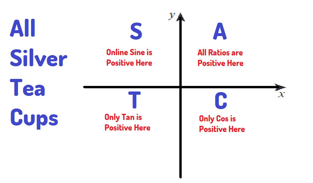
The Trigonometric Ratios and their Quadrant relationship
Question
Trigonometric Ratios of Acute Angles
Problem a: \( \sin 140^\circ \)
Step 1: Recognize that \( 140^\circ \) is in the second quadrant.
In the second quadrant, the sine function is positive, and we can relate \( \sin 140^\circ \) to an acute angle.
Step 2: Find the reference angle.
The reference angle for any angle in the second quadrant is calculated as: \[ \text{Reference angle} = 180^\circ - \theta \] For \( 140^\circ \): \[ \text{Reference angle} = 180^\circ - 140^\circ = 40^\circ \]
Step 3: Express \( \sin 140^\circ \) in terms of the acute angle.
Since sine is positive in the second quadrant: \[ \sin 140^\circ = \sin 40^\circ \]
Problem b: \( \cos (-130^\circ) \)
Step 1: Recognize that \( -130^\circ \) is a negative angle.
Negative angles are measured clockwise from the positive x-axis.
Step 2: Convert \( \cos (-130^\circ) \) to a positive angle.
To find the equivalent positive angle, we add \( 360^\circ \): \[ -130^\circ + 360^\circ = 230^\circ \]
Step 3: Recognize that \( 230^\circ \) is in the third quadrant.
In the third quadrant, cosine is negative.
Step 4: Find the reference angle.
The reference angle for angles in the third quadrant is: \[ \text{Reference angle} = \theta - 180^\circ \] For \( 230^\circ \): \[ \text{Reference angle} = 230^\circ - 180^\circ = 50^\circ \]
Step 5: Express \( \cos (-130^\circ) \) in terms of the acute angle.
Since cosine is negative in the third quadrant: \[ \cos (-130^\circ) = \cos 230^\circ = -\cos 50^\circ \]
Final Answers:
\[ \sin 140^\circ = \sin 40^\circ \] \[ \cos (-130^\circ) = -\cos 50^\circ \]
Question
Given: \( \cos \theta = \frac{-3}{5} \) and \( 180^\circ \leq \theta \leq 270^\circ \)
Find the values of \( \sin \theta \) and \( \tan \theta \).
Step 1: Recognize that \( \theta \) is in the third quadrant.
The given range \( 180^\circ \leq \theta \leq 270^\circ \) indicates that \( \theta \) is in the third quadrant, where cosine is negative and sine is also negative.
Step 2: Use the Pythagorean identity to find \( \sin \theta \).
We use the identity \( \sin^2 \theta + \cos^2 \theta = 1 \): \[ \sin^2 \theta = 1 - \cos^2 \theta = 1 - \left( \frac{-3}{5} \right)^2 = 1 - \frac{9}{25} = \frac{16}{25} \] Therefore: \[ \sin \theta = -\frac{4}{5} \] (Since sine is negative in the third quadrant)
Step 3: Find \( \tan \theta \).
We know that \( \tan \theta = \frac{\sin \theta}{\cos \theta} \). Using the values of \( \sin \theta = \frac{-4}{5} \) and \( \cos \theta = \frac{-3}{5} \): \[ \tan \theta = \frac{-4/5}{-3/5} = \frac{4}{3} \]
Final Answers:
\[ \sin \theta = -\frac{4}{5} \] \[ \tan \theta = \frac{4}{3} \]
Problem a: \( \sin 120^\circ \), Without using a calculator, find the exact values
Step 1: Recognize that \( 120^\circ \) is in the second quadrant.
In the second quadrant, sine is positive, and cosine is negative.
Step 2: Find the reference angle.
The reference angle is: \[ \text{Reference angle} = 180^\circ - 120^\circ = 60^\circ \]
Step 3: Use the known value of \( \sin 60^\circ \).
Since sine is positive in the second quadrant: \[ \sin 120^\circ = \sin 60^\circ = \frac{\sqrt{3}}{2} \]
Problem b: \( \cos \frac{7\pi}{6} \) Without using a calculator, find the exact values
Step 1: Recognize that \( \frac{7\pi}{6} \) is in the third quadrant.
The angle \( \frac{7\pi}{6} \) is greater than \( \pi \) (i.e., \( 180^\circ \)) and less than \( \frac{3\pi}{2} \) (i.e., \( 270^\circ \)), placing it in the third quadrant where cosine is negative.
Step 2: Find the reference angle.
The reference angle is: \[ \text{Reference angle} = \frac{7\pi}{6} - \pi = \frac{\pi}{6} \]
Step 3: Use the known value of \( \cos \frac{\pi}{6} \) and apply the quadrant sign.
Since cosine is negative in the third quadrant: \[ \cos \frac{7\pi}{6} = -\cos \frac{\pi}{6} = -\frac{\sqrt{3}}{2} \]
Final Answers:
\[ \sin 120^\circ = \frac{\sqrt{3}}{2} \] \[ \cos \frac{7\pi}{6} = -\frac{\sqrt{3}}{2} \]
Trigonometric Solutions
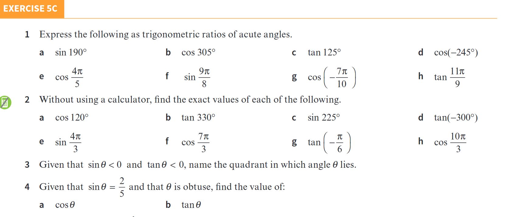
Question 1: Express as trigonometric ratios of acute angles
a. \( \sin 190^\circ \)
\( 190^\circ \) is in the third quadrant where sine is negative. The reference angle is: \[ 190^\circ - 180^\circ = 10^\circ \] Therefore: \[ \sin 190^\circ = -\sin 10^\circ \]
b. \( \cos 305^\circ \)
\( 305^\circ \) is in the fourth quadrant where cosine is positive. The reference angle is: \[ 360^\circ - 305^\circ = 55^\circ \] Therefore: \[ \cos 305^\circ = \cos 55^\circ \]
c. \( \tan 125^\circ \)
\( 125^\circ \) is in the second quadrant where tangent is negative. The reference angle is: \[ 180^\circ - 125^\circ = 55^\circ \] Therefore: \[ \tan 125^\circ = -\tan 55^\circ \]
d. \( \cos (-245^\circ) \)
First, convert the negative angle to a positive one by adding \( 360^\circ \): \[ -245^\circ + 360^\circ = 115^\circ \] \( 115^\circ \) is in the second quadrant where cosine is negative. The reference angle is: \[ 180^\circ - 115^\circ = 65^\circ \] Therefore: \[ \cos (-245^\circ) = -\cos 65^\circ \]
e. \( \cos \frac{4\pi}{5} \)
\( \frac{4\pi}{5} \) is in the second quadrant where cosine is negative. The reference angle is: \[ \pi - \frac{4\pi}{5} = \frac{\pi}{5} \] Therefore: \[ \cos \frac{4\pi}{5} = -\cos \frac{\pi}{5} \]
f. \( \sin \frac{9\pi}{8} \)
\( \frac{9\pi}{8} \) is in the third quadrant where sine is negative. The reference angle is: \[ \frac{9\pi}{8} - \pi = \frac{\pi}{8} \] Therefore: \[ \sin \frac{9\pi}{8} = -\sin \frac{\pi}{8} \]
g. \( \cos \left( \frac{-7\pi}{10} \right) \)
First, convert the negative angle to a positive one by adding \( 2\pi \): \[ \frac{-7\pi}{10} + 2\pi = \frac{13\pi}{10} \] \( \frac{13\pi}{10} \) is in the fourth quadrant where cosine is positive. The reference angle is: \[ 2\pi - \frac{13\pi}{10} = \frac{\pi}{10} \] Therefore: \[ \cos \left( \frac{-7\pi}{10} \right) = \cos \frac{\pi}{10} \]
h. \( \tan \frac{11\pi}{9} \)
\( \frac{11\pi}{9} \) is in the third quadrant where tangent is positive. The reference angle is: \[ \frac{11\pi}{9} - \pi = \frac{2\pi}{9} \] Therefore: \[ \tan \frac{11\pi}{9} = \tan \frac{2\pi}{9} \]
Question 2: Find exact values without using a calculator
a. \( \cos 120^\circ \)
\( 120^\circ \) is in the second quadrant where cosine is negative. The reference angle is: \[ 180^\circ - 120^\circ = 60^\circ \] Therefore: \[ \cos 120^\circ = -\cos 60^\circ = -\frac{1}{2} \]
b. \( \tan 330^\circ \)
\( 330^\circ \) is in the fourth quadrant where tangent is negative. The reference angle is: \[ 360^\circ - 330^\circ = 30^\circ \] Therefore: \[ \tan 330^\circ = -\tan 30^\circ = -\frac{1}{\sqrt{3}} \]
c. \( \sin 225^\circ \)
\( 225^\circ \) is in the third quadrant where sine is negative. The reference angle is: \[ 225^\circ - 180^\circ = 45^\circ \] Therefore: \[ \sin 225^\circ = -\sin 45^\circ = -\frac{\sqrt{2}}{2} \]
d. \( \tan (-300^\circ) \)
Convert the negative angle to a positive angle by adding \( 360^\circ \): \[ -300^\circ + 360^\circ = 60^\circ \] \( 60^\circ \) is in the first quadrant where tangent is positive. Therefore: \[ \tan (-300^\circ) = \tan 60^\circ = \sqrt{3} \]
e. \( \sin \frac{4\pi}{3} \)
\( \frac{4\pi}{3} \) is in the third quadrant where sine is negative. The reference angle is: \[ \frac{4\pi}{3} - \pi = \frac{\pi}{3} \] Therefore: \[ \sin \frac{4\pi}{3} = -\sin \frac{\pi}{3} = -\frac{\sqrt{3}}{2} \]
f. \( \cos \frac{7\pi}{3} \)
Convert \( \frac{7\pi}{3} \) to a standard angle by subtracting \( 2\pi \): \[ \frac{7\pi}{3} - 2\pi = \frac{\pi}{3} \] \( \frac{\pi}{3} \) is in the first quadrant where cosine is positive. Therefore: \[ \cos \frac{7\pi}{3} = \cos \frac{\pi}{3} = \frac{1}{2} \]
g. \( \tan \left( \frac{-\pi}{6} \right) \)
Convert the negative angle to a positive one by adding \( 2\pi \): \[ \frac{-\pi}{6} + 2\pi = \frac{11\pi}{6} \] \( \frac{11\pi}{6} \) is in the fourth quadrant where tangent is negative. The reference angle is: \[ 2\pi - \frac{11\pi}{6} = \frac{\pi}{6} \] Therefore: \[ \tan \left( \frac{-\pi}{6} \right) = -\tan \frac{\pi}{6} = -\frac{1}{\sqrt{3}} \]
h. \( \cos \frac{10\pi}{3} \)
Convert \( \frac{10\pi}{3} \) to a standard angle by subtracting \( 2\pi \): \[ \frac{10\pi}{3} - 2\pi = \frac{4\pi}{3} \] \( \frac{4\pi}{3} \) is in the third quadrant where cosine is negative. The reference angle is: \[ \frac{4\pi}{3} - \pi = \frac{\pi}{3} \] Therefore: \[ \cos \frac{10\pi}{3} = -\cos \frac{\pi}{3} = -\frac{1}{2} \]
Question 3: Determine the quadrant
Given \( \sin \theta < 0 \) and \( \tan \theta < 0 \)
\( \sin \theta < 0 \) indicates that \( \theta \) is either in the third or fourth quadrant. \( \tan \theta < 0 \) indicates that \( \theta \) is either in the second or fourth quadrant. The only quadrant where both conditions are true is the fourth quadrant.
Question 4: Given \( \sin \theta = \frac{2}{5} \) and \( \theta \) is obtuse
a. Find \( \cos \theta \)
Using the identity \( \sin^2 \theta + \cos^2 \theta = 1 \): \[ \cos^2 \theta = 1 - \sin^2 \theta = 1 - \left( \frac{2}{5} \right)^2 = 1 - \frac{4}{25} = \frac{21}{25} \] Therefore: \[ \cos \theta = -\frac{\sqrt{21}}{5} \] (since \( \theta \) is obtuse, cosine is negative)
b. Find \( \tan \theta \)
We know that \( \tan \theta = \frac{\sin \theta}{\cos \theta} \): \[ \tan \theta = \frac{\frac{2}{5}}{-\frac{\sqrt{21}}{5}} = -\frac{2}{\sqrt{21}} \]
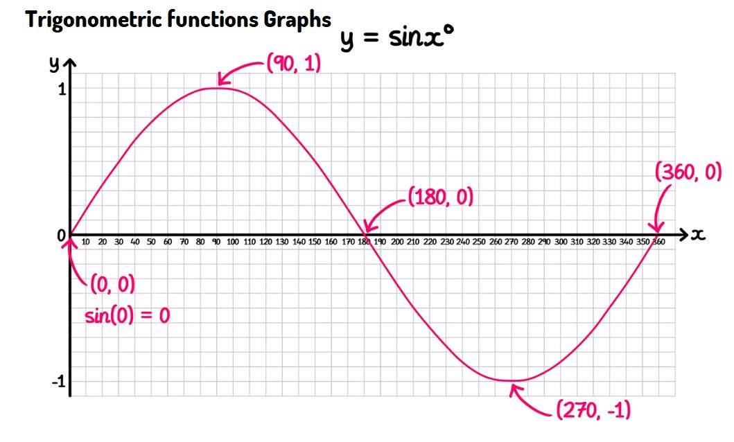
Graphing Trigonometric Functions - \( y = \sin{x} \)
1. Introduction
The sine function, \( y = \sin{x} \), is one of the basic trigonometric functions that shows a periodic wave-like pattern. It is important to understand how to graph this function to analyze its behavior and applications in real-life scenarios, such as sound waves, light waves, and other oscillating phenomena.
2. Key Characteristics of \( y = \sin{x} \)
- The sine function is periodic with a period of \( 360^\circ \) (or \( 2\pi \) radians).
- The function oscillates between a maximum value of \( 1 \) and a minimum value of \( -1 \).
- The graph of \( y = \sin{x} \) crosses the x-axis at \( 0^\circ \), \( 180^\circ \), and \( 360^\circ \), corresponding to points where \( \sin{x} = 0 \).
- The function reaches its maximum value of \( 1 \) at \( 90^\circ \) and its minimum value of \( -1 \) at \( 270^\circ \).
3. Step-by-Step Graphing of \( y = \sin{x} \)
To plot the graph of \( y = \sin{x} \), follow these steps:
- Step 1: Identify Key Points
Mark the key points where the sine function reaches specific values:
- \( (0^\circ, 0) \): Start at the origin where \( \sin{0^\circ} = 0 \).
- \( (90^\circ, 1) \): The sine function reaches its maximum value of \( 1 \).
- \( (180^\circ, 0) \): The sine function returns to zero.
- \( (270^\circ, -1) \): The sine function reaches its minimum value of \( -1 \).
- \( (360^\circ, 0) \): The sine function completes one period and returns to zero.
- Step 2: Plot the Points on a Graph
Draw a set of axes with the x-axis representing the angle in degrees (from \( 0^\circ \) to \( 360^\circ \)), and the y-axis representing the sine values (from \( -1 \) to \( 1 \)). Plot the points identified in Step 1.
- Step 3: Draw a Smooth Curve Through the Points
Connect the points with a smooth, wave-like curve to complete the graph of one period of the sine function.
4. Explanation
5. Additional Notes
The sine function graph repeats every \( 360^\circ \), meaning it is a periodic function. This periodicity makes sine functions useful in modeling oscillatory behavior in real-world applications, such as sound waves, light waves, and alternating current electricity.
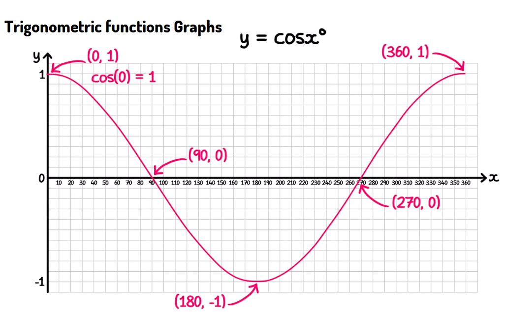
Graphing Trigonometric Functions - \( y = \cos{x} \)
1. Introduction
The cosine function, \( y = \cos{x} \), is one of the fundamental trigonometric functions. It exhibits a wave-like pattern, oscillating between maximum and minimum values periodically. Understanding how to graph this function is crucial in analyzing various real-world phenomena like sound waves, alternating currents, and other cyclic behaviors.
2. Key Characteristics of \( y = \cos{x} \)
- The cosine function is periodic with a period of \( 360^\circ \) (or \( 2\pi \) radians).
- The function oscillates between a maximum value of \( 1 \) and a minimum value of \( -1 \).
- The graph of \( y = \cos{x} \) crosses the x-axis at \( 90^\circ \) and \( 270^\circ \), corresponding to points where \( \cos{x} = 0 \).
- The function reaches its maximum value of \( 1 \) at \( 0^\circ \) and \( 360^\circ \), and its minimum value of \( -1 \) at \( 180^\circ \).
3. Step-by-Step Graphing of \( y = \cos{x} \)
To plot the graph of \( y = \cos{x} \), follow these steps:
- Step 1: Identify Key Points
Mark the key points where the cosine function reaches specific values:
- \( (0^\circ, 1) \): Start at the maximum value where \( \cos{0^\circ} = 1 \).
- \( (90^\circ, 0) \): The cosine function crosses the x-axis.
- \( (180^\circ, -1) \): The cosine function reaches its minimum value of \( -1 \).
- \( (270^\circ, 0) \): The cosine function crosses the x-axis again.
- \( (360^\circ, 1) \): The cosine function completes one period and returns to its maximum value.
- Step 2: Plot the Points on a Graph
Draw a set of axes with the x-axis representing the angle in degrees (from \( 0^\circ \) to \( 360^\circ \)), and the y-axis representing the cosine values (from \( -1 \) to \( 1 \)). Plot the points identified in Step 1.
- Step 3: Draw a Smooth Curve Through the Points
Connect the points with a smooth, wave-like curve to complete the graph of one period of the cosine function.
4. Explanation
5. Additional Notes
The cosine function graph repeats every \( 360^\circ \), meaning it is a periodic function. This periodicity makes cosine functions useful in modeling oscillatory behavior in various fields such as physics, engineering, and signal processing.
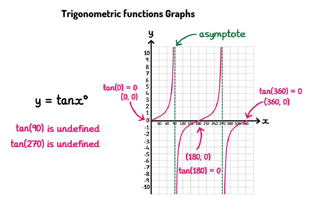
Graphing Trigonometric Functions - \( y = \tan{x} \)
1. Introduction
The tangent function, \( y = \tan{x} \), is another fundamental trigonometric function. Unlike sine and cosine functions, the tangent function exhibits vertical asymptotes where it is undefined, making its graph quite different. It is periodic with a period of \( 180^\circ \) (or \( \pi \) radians), and understanding how to graph this function is essential for analyzing various oscillatory behaviors and wave patterns.
2. Key Characteristics of \( y = \tan{x} \)
- The tangent function has a period of \( 180^\circ \) (or \( \pi \) radians).
- The function oscillates between negative and positive infinity, with vertical asymptotes where the function is undefined.
- The vertical asymptotes occur at \( 90^\circ \), \( 270^\circ \), etc., where \( \tan{x} \) is undefined.
- The graph of \( y = \tan{x} \) crosses the x-axis at multiples of \( 180^\circ \), corresponding to points where \( \tan{x} = 0 \).
- The function repeats every \( 180^\circ \), making it periodic with this interval.
3. Step-by-Step Graphing of \( y = \tan{x} \)
To plot the graph of \( y = \tan{x} \), follow these steps:
- Step 1: Identify Key Points
Mark the key points where the tangent function reaches specific values:
- \( (0^\circ, 0) \): Start at the origin where \( \tan{0^\circ} = 0 \).
- \( (180^\circ, 0) \): The tangent function returns to zero after one period.
- \( (360^\circ, 0) \): The function completes two periods and returns to zero again.
- Vertical asymptotes occur at \( 90^\circ \), \( 270^\circ \), etc., where the function is undefined.
- Step 2: Plot the Points on a Graph
Draw a set of axes with the x-axis representing the angle in degrees (from \( 0^\circ \) to \( 360^\circ \)), and the y-axis representing the tangent values. Plot the key points and mark the vertical asymptotes.
- Step 3: Draw a Smooth Curve Approaching the Asymptotes
Connect the points with a smooth curve that approaches the vertical asymptotes. The graph will show an increasing trend from negative infinity to positive infinity between the asymptotes.
4. Explanation
5. Additional Notes
The tangent function graph repeats every \( 180^\circ \), meaning it is a periodic function with vertical asymptotes where the function is undefined. This behavior is useful in modeling oscillatory behavior and wave patterns in fields such as physics, engineering, and signal processing.
Transformations of Trigonometric Functions - \( y = a \sin{x} \)
1. Introduction
Transformations of trigonometric functions allow us to manipulate the basic shape of their graphs. These transformations can include scaling, shifting, and reflecting the graph. In this case, we will explore the transformation \( y = a \sin{x} \), where the parameter \( a \) affects the amplitude of the sine function.
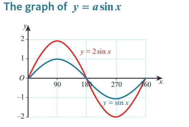
2. Understanding the Transformation \( y = a \sin{x} \)
- In the equation \( y = a \sin{x} \), the parameter \( a \) is known as the amplitude.
- The amplitude determines how much the graph stretches or compresses vertically.
- When \( a > 1 \), the graph stretches vertically, making the peaks and troughs higher and lower.
- When \( 0 < a < 1 \), the graph compresses vertically, resulting in lower peaks and shallower troughs.
- If \( a < 0 \), the graph is reflected across the x-axis, in addition to being stretched or compressed.
3. Step-by-Step Graphing of \( y = a \sin{x} \)
To graph \( y = a \sin{x} \), follow these steps:
- Step 1: Identify Key Points for \( y = \sin{x} \)
Plot the basic sine wave, \( y = \sin{x} \), which passes through the points:
- \( (0^\circ, 0) \), \( (90^\circ, 1) \), \( (180^\circ, 0) \), \( (270^\circ, -1) \), \( (360^\circ, 0) \).
- Step 2: Apply the Transformation by Scaling the Amplitude
Multiply the y-values of each key point by the factor \( a \). For example, if \( a = 2 \), the points become:
- \( (0^\circ, 0) \), \( (90^\circ, 2) \), \( (180^\circ, 0) \), \( (270^\circ, -2) \), \( (360^\circ, 0) \).
- Step 3: Draw the New Sine Wave
Connect the transformed points with a smooth curve, showing the stretched or compressed sine wave based on the value of \( a \).
4. Explanation
5. Additional Notes
The transformation \( y = a \sin{x} \) affects the vertical stretching or compression of the sine wave. The period remains unchanged at \( 360^\circ \). This transformation can be applied similarly to other trigonometric functions like cosine and tangent.
Transformations of Trigonometric Functions - \( y = \sin(ax) \)
1. Introduction
The transformation \( y = \sin(ax) \) modifies the frequency of the sine wave. The parameter \( a \) affects the number of cycles that the sine function completes over a given interval. This transformation changes the period of the function but does not affect the amplitude.
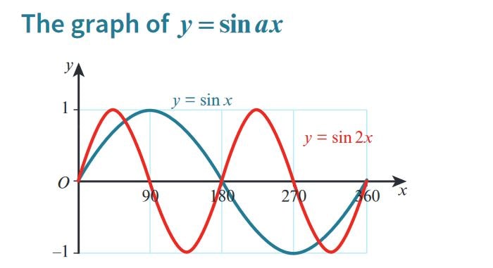
2. Understanding the Transformation \( y = \sin(ax) \)
- In the equation \( y = \sin(ax) \), the parameter \( a \) is a frequency multiplier.
- The frequency of the sine wave increases as \( a \) increases, meaning more cycles are completed within the same interval.
- The period of the sine function is calculated as \( \frac{360^\circ}{a} \) (or \( \frac{2\pi}{a} \) radians).
- If \( a > 1 \), the sine wave completes more cycles, and the graph becomes more "compressed" horizontally.
- If \( 0 < a < 1 \), the sine wave completes fewer cycles, and the graph becomes "stretched" horizontally.
3. Step-by-Step Graphing of \( y = \sin(ax) \)
To graph \( y = \sin(ax) \), follow these steps:
- Step 1: Identify the Period of the Function
The period of the sine function is given by \( \frac{360^\circ}{a} \). For example, if \( a = 2 \), the period becomes \( \frac{360^\circ}{2} = 180^\circ \).
- Step 2: Plot Key Points Over One Period
Plot the basic sine wave over the calculated period. For \( y = \sin(2x) \), the key points would be:
- \( (0^\circ, 0) \), \( (45^\circ, 1) \), \( (90^\circ, 0) \), \( (135^\circ, -1) \), \( (180^\circ, 0) \).
- Step 3: Repeat the Pattern for Additional Periods
Continue plotting the wave beyond the first period to complete the graph over the desired interval.
4. Explanation
5. Additional Notes
The transformation \( y = \sin(ax) \) affects the horizontal compression or stretching of the sine wave but does not change its amplitude. The frequency multiplier \( a \) alters how many complete cycles fit within \( 360^\circ \) or \( 2\pi \) radians.
Transformations of Trigonometric Functions - \( y = a + \sin{x} \)
1. Introduction
The transformation \( y = a + \sin{x} \) represents a vertical shift of the sine function. The parameter \( a \) determines how much the graph shifts up or down along the y-axis. Understanding this transformation helps in analyzing periodic behavior with adjusted baselines.
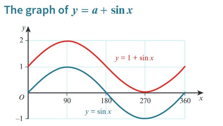
2. Understanding the Transformation \( y = a + \sin{x} \)
- In the equation \( y = a + \sin{x} \), the parameter \( a \) causes a vertical shift of the sine wave.
- If \( a > 0 \), the graph shifts upward by \( a \) units.
- If \( a < 0 \), the graph shifts downward by \( |a| \) units.
- The amplitude remains unchanged, and the period of the function is still \( 360^\circ \) (or \( 2\pi \) radians).
- This transformation changes the midline of the sine wave from \( y = 0 \) to \( y = a \).
3. Step-by-Step Graphing of \( y = a + \sin{x} \)
To graph \( y = a + \sin{x} \), follow these steps:
- Step 1: Plot the Basic Sine Wave \( y = \sin{x} \)
Start by plotting the basic sine wave, which passes through points such as:
- \( (0^\circ, 0) \), \( (90^\circ, 1) \), \( (180^\circ, 0) \), \( (270^\circ, -1) \), \( (360^\circ, 0) \).
- Step 2: Apply the Vertical Shift
Shift the entire graph vertically by adding \( a \) to each y-coordinate. For example, if \( a = 1 \), the points become:
- \( (0^\circ, 1) \), \( (90^\circ, 2) \), \( (180^\circ, 1) \), \( (270^\circ, 0) \), \( (360^\circ, 1) \).
The midline of the graph shifts from \( y = 0 \) to \( y = 1 \).
- Step 3: Draw the New Sine Wave
Connect the new points with a smooth curve to represent the vertically shifted sine wave.
4. Explanation
5. Additional Notes
The transformation \( y = a + \sin{x} \) shifts the sine wave vertically by \( a \) units. This is useful for modeling real-life phenomena where the baseline or equilibrium position is not zero.
Transformations of Trigonometric Functions - \( y = \sin(x + a) \)
1. Introduction
The transformation \( y = \sin(x + a) \) represents a horizontal shift of the sine function. The parameter \( a \) determines the direction and magnitude of the shift along the x-axis. This transformation is often referred to as a phase shift in trigonometry.
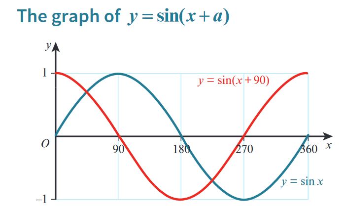
2. Understanding the Transformation \( y = \sin(x + a) \)
- In the equation \( y = \sin(x + a) \), the parameter \( a \) causes a horizontal shift of the sine wave.
- If \( a > 0 \), the graph shifts to the left by \( a \) units (i.e., in the negative x-direction).
- If \( a < 0 \), the graph shifts to the right by \( |a| \) units (i.e., in the positive x-direction).
- The amplitude and period of the function remain unchanged.
- The phase shift results in the movement of key points along the x-axis.
3. Step-by-Step Graphing of \( y = \sin(x + a) \)
To graph \( y = \sin(x + a) \), follow these steps:
- Step 1: Plot the Basic Sine Wave \( y = \sin{x} \)
Start by plotting the basic sine wave, which passes through points such as:
- \( (0^\circ, 0) \), \( (90^\circ, 1) \), \( (180^\circ, 0) \), \( (270^\circ, -1) \), \( (360^\circ, 0) \).
- Step 2: Apply the Horizontal Shift
Shift the entire graph horizontally by \( a \) units. For example, if \( a = 90^\circ \), shift all points 90 degrees to the left:
- The new points become: \( (-90^\circ, 0) \), \( (0^\circ, 1) \), \( (90^\circ, 0) \), \( (180^\circ, -1) \), \( (270^\circ, 0) \).
- Step 3: Draw the New Sine Wave
Connect the new points with a smooth curve to represent the horizontally shifted sine wave.
4. Explanation
5. Additional Notes
The transformation \( y = \sin(x + a) \) shifts the sine wave horizontally by \( a \) units. This type of transformation is used to model periodic phenomena where the starting point of the cycle is shifted from the usual position.
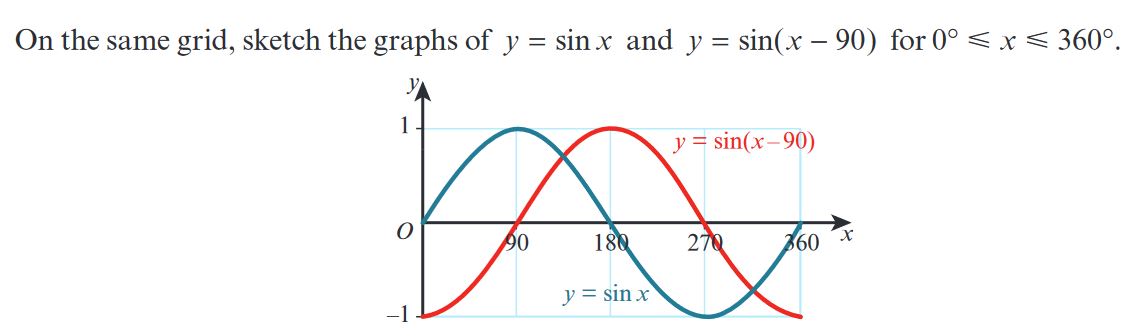
Transformations of Trigonometric Functions - \( y = \sin{x} \) and \( y = \sin(x - 90) \)
1. Introduction
In this exercise, we will explore the transformation of the sine function \( y = \sin{x} \) to \( y = \sin(x - 90) \). This transformation represents a horizontal shift of the graph. Specifically, the parameter \( -90 \) shifts the graph to the right by 90 degrees.
2. Understanding the Transformation \( y = \sin(x - 90) \)
- The equation \( y = \sin(x - 90) \) involves a horizontal shift of the sine wave.
- The term \( -90 \) indicates a shift to the right by 90 degrees.
- This transformation does not change the amplitude or period of the sine function; it only shifts the graph along the x-axis.
- The original sine function \( y = \sin{x} \) will be translated by the vector \( \begin{pmatrix} 90 \\ 0 \end{pmatrix} \), moving all key points 90 degrees to the right.
3. Step-by-Step Graphing of \( y = \sin{x} \) and \( y = \sin(x - 90) \)
To graph \( y = \sin{x} \) and \( y = \sin(x - 90) \), follow these steps:
- Step 1: Plot the Basic Sine Wave \( y = \sin{x} \)
Start by plotting the basic sine wave, which passes through points such as:
- \( (0^\circ, 0) \), \( (90^\circ, 1) \), \( (180^\circ, 0) \), \( (270^\circ, -1) \), \( (360^\circ, 0) \).
- Step 2: Apply the Horizontal Shift for \( y = \sin(x - 90) \)
Shift all points of the original sine wave to the right by 90 degrees:
- The new points for \( y = \sin(x - 90) \) are: \( (90^\circ, 0) \), \( (180^\circ, 1) \), \( (270^\circ, 0) \), \( (360^\circ, -1) \), \( (450^\circ, 0) \).
- Step 3: Draw Both Graphs on the Same Grid
Plot both \( y = \sin{x} \) and \( y = \sin(x - 90) \) on the same grid to visualize the transformation. The graph of \( y = \sin(x - 90) \) will appear as the original sine wave shifted to the right.
4. Explanation
5. Additional Notes
The transformation from \( y = \sin{x} \) to \( y = \sin(x - 90) \) is a horizontal translation of the sine wave. This shift is used to model scenarios where the phase or starting point of a periodic function changes.
Graphing Trigonometric Functions - \( y = 2 \cos(x + 90) + 1 \)
1. Introduction
We will sketch the graph of the function \( y = 2 \cos(x + 90) + 1 \). This function involves three transformations: a horizontal shift, a vertical scaling (amplitude change), and a vertical shift.
2. Understanding the Transformations
- The equation \( y = 2 \cos(x + 90) + 1 \) includes:
- Amplitude Change: The factor 2 in front of the cosine function increases the amplitude from 1 to 2. The graph will oscillate between -2 and 2.
- Horizontal Shift: The term \( (x + 90) \) shifts the graph 90 degrees to the left.
- Vertical Shift: The "+1" shifts the entire graph up by 1 unit, changing the midline from \( y = 0 \) to \( y = 1 \).
3. Step-by-Step Graphing of \( y = 2 \cos(x + 90) + 1 \)
To sketch the graph, follow these steps:
- Step 1: Plot the Basic Cosine Function \( y = \cos{x} \)
Start with the basic cosine function, which oscillates between 1 and -1, with key points:
- \( (0^\circ, 1) \), \( (90^\circ, 0) \), \( (180^\circ, -1) \), \( (270^\circ, 0) \), \( (360^\circ, 1) \).
- Step 2: Apply the Amplitude Change to \( y = 2 \cos{x} \)
Multiply each y-coordinate by 2, resulting in new key points:
- \( (0^\circ, 2) \), \( (90^\circ, 0) \), \( (180^\circ, -2) \), \( (270^\circ, 0) \), \( (360^\circ, 2) \).
- Step 3: Apply the Horizontal Shift to \( y = 2 \cos(x + 90) \)
Shift all points 90 degrees to the left, resulting in new key points:
- \( (-90^\circ, 2) \), \( (0^\circ, 0) \), \( (90^\circ, -2) \), \( (180^\circ, 0) \), \( (270^\circ, 2) \).
- Step 4: Apply the Vertical Shift to \( y = 2 \cos(x + 90) + 1 \)
Add 1 to each y-coordinate, resulting in the final key points:
- \( (-90^\circ, 3) \), \( (0^\circ, 1) \), \( (90^\circ, -1) \), \( (180^\circ, 1) \), \( (270^\circ, 3) \).
The new midline is \( y = 1 \), and the graph oscillates between -1 and 3.
4. Explanation
5. Additional Notes
The function \( y = 2 \cos(x + 90) + 1 \) combines multiple transformations, resulting in a shifted, scaled, and vertically adjusted cosine wave. Understanding each transformation step-by-step allows us to sketch the graph accurately.
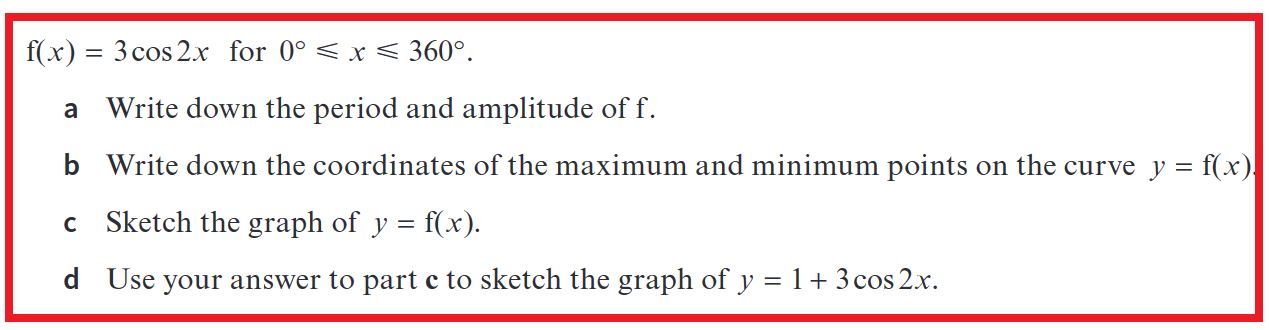
Trigonometric Function - \( f(x) = 3 \cos 2x \)
a. Write down the period and amplitude of \( f \).
The general form of the cosine function is \( f(x) = a \cos(bx) \), where:
- \( |a| \) represents the amplitude.
- The period is given by \( \frac{360^\circ}{b} \).
For \( f(x) = 3 \cos 2x \), we have:
- \( a = 3 \), so the amplitude is \( 3 \).
- \( b = 2 \), so the period is \( \frac{360^\circ}{2} = 180^\circ \).
Therefore, the amplitude is 3, and the period is \( 180^\circ \).
b. Write down the coordinates of the maximum and minimum points on the curve \( y = f(x) \).
For \( f(x) = 3 \cos 2x \), the maximum value is 3, and the minimum value is -3.
- The cosine function starts at its maximum value when \( x = 0^\circ \), so the first maximum point is \( (0^\circ, 3) \).
- The first minimum occurs at \( 90^\circ \), so the coordinates are \( (90^\circ, -3) \).
- The next maximum occurs at \( 180^\circ \), with coordinates \( (180^\circ, 3) \).
- The next minimum occurs at \( 270^\circ \), with coordinates \( (270^\circ, -3) \).
- Finally, the curve reaches its maximum again at \( 360^\circ \), with coordinates \( (360^\circ, 3) \).
c. Sketch the graph of \( y = f(x) \).
The graph of \( y = 3 \cos 2x \) will have an amplitude of 3 and a period of \( 180^\circ \). Key points to plot are:
- \( (0^\circ, 3) \) - Maximum
- \( (90^\circ, -3) \) - Minimum
- \( (180^\circ, 3) \) - Maximum
- \( (270^\circ, -3) \) - Minimum
- \( (360^\circ, 3) \) - Maximum
Connect these points with a smooth wave to complete the graph.
d. Use your answer to part c to sketch the graph of \( y = 1 + 3 \cos 2x \).
The function \( y = 1 + 3 \cos 2x \) can be considered as the graph of \( y = 3 \cos 2x \) shifted up by 1 unit.
- The new maximum value is \( 3 + 1 = 4 \).
- The new minimum value is \( -3 + 1 = -2 \).
- The midline of the graph is now at \( y = 1 \) instead of \( y = 0 \).
- Key points to plot are:
- \( (0^\circ, 4) \) - Maximum
- \( (90^\circ, -2) \) - Minimum
- \( (180^\circ, 4) \) - Maximum
- \( (270^\circ, -2) \) - Minimum
- \( (360^\circ, 4) \) - Maximum
Connect these points with a smooth wave to complete the graph of \( y = 1 + 3 \cos 2x \).